Summary

This document describes the 3rd prize solution to the Second National Data Science Bowl hosted by Kaggle.com. The goal of the challenge was to perform automatic volume measurement of the left ventricle based on MRI images. I will skip the description of the challenge since it has already been described on the Kaggle competition page and this blog post of the #2. My solution relied heavily on image segmentation with a neural network architecture called U-nets.

The plan

After the last retinopathy challenge I really got a taste for solving medical problems. Therefore I was very excited about this competition. Just to get a feeling for the case I decided to manually segment a few patients and to compute the volume on paper. With the information from the DICOM files (pixel spacing, image location etc) one could go directly from pixels to milliliters. Without exaclty knowing how to determine which areas were part of the left ventricle (LV) I roughly got an error of ~10ml. My conclusion was that if I could learn the computer how to segment the LV, it would result in a very good score. Below is the idealized schema for the envisioned solution.

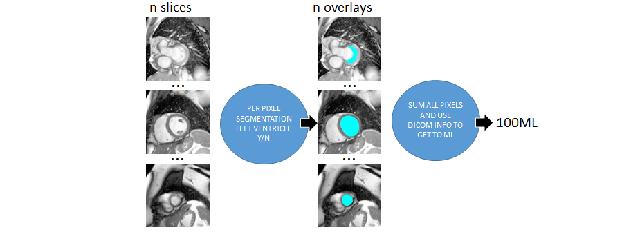Figure 1. The idealized version of my approach

Of course things turned out to be a bit harder than expected. First of all, the data was far from perfect. Second it was very hard to find information on how exactly one can determine left ventricle area on MRI images. I decided to manually label some images as good as I could possibly do and extend my system with a data cleaning part and a calibration step. The calibration step uses the provided volumes in the traindata to correct for systematic mistakes made with labeling. In the next paragraph I will try to discuss every step of the complete solution.

Preprocessing

The MRI images were provided in the DICOM format. The DICOM files contained an MRI scan image and lots of metadata. The preprocessing consisted of two paths. The first path was to extract the images from the file and make them uniform and easier to see and process. All images were taken at different scales (reflected in the pixel-spacing property). My hunch was that this is done to get more uniform pictures of the heart. Small hearts would be zoomed in and bigger hart would be zoomed out. By just looking at the images I still saw a lot of variance and the picture just did not look very uniform. Therefore I decided to scale every image by the pixel-spacing^2 factor. The result was that for every image 1 pixel respresented the same area. After scaling the images I noted that the heart was always bounded by a 180x180 area. Usually it’s good to leave out irrelevant information for picking up signal by the machine learning algorithm. Next to this, it also helps for processing speed. Therefore it was decided to crop all images to 180x180. Last but not least, for my own viewing pleasure and to hopefully help the machine learning algorithm I applied contrast stretching to the images using CLAHE (tilesize 1x1).

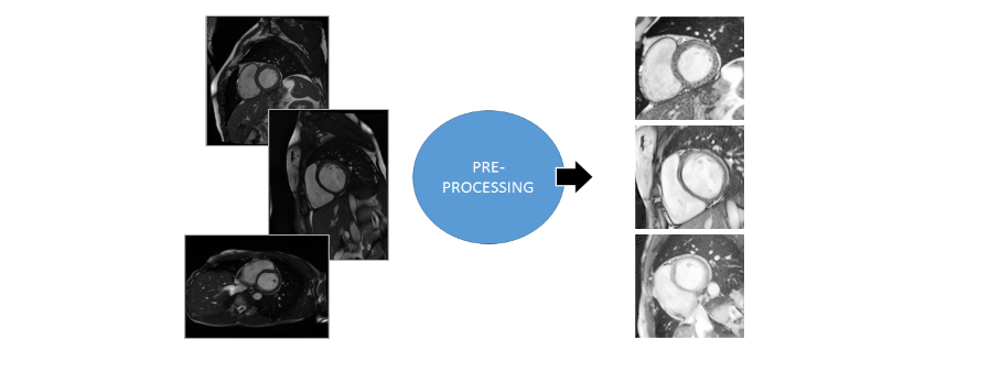Figure 2. Image preprocessing step

The second preprocessing path was to find useful metadata fields that could be used for the data-cleaning and calibration step. Examples of interesting features were age, sex, slice-count, slice-distance, image-orientation, scan-time, image-size and a few others. The features were stored in a separate csv file for later use.

Hand labeling

The traindata of the competition only contained the final determined volumes of the left ventricle. There was no information on how this volume was obtained. There was the possibility of using the Sunnybrook dataset but the cases in that set were much more simple than the cases I encountered in the DICOM files. Of course I was thinking of using a convolutional neural network (CNN) for the image segmentation. CNN’s are great but they need a lot of traindata. Luckily I already had an overlay-drawing tool that I once built for an earlier project. I decided to label 100 patients with this tool. For every patient I took frame 1 (usually diastole) and frame 12 (usually systole).

Since every patient had around 10 slices that meant that I had to label around 2000 images. Once I got the hang of it using my tool I was able to label around 1 patient per minute. During the labeling I encountered many confusing cases that I still don’t know how to label. I scanned youtube and many papers but there were no definate answers on the internet. In the end I decided to at least be consistent. If I would be consistent then in a later stage I could brush out systematic errors during the calibration phase. Below are a number of situations that were encountered.

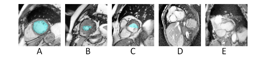Figure 3. A. Easy. B. Harder since it was unclear if only the white (bloodpool) should be annoted or that the tissue should be interpreted like sponge C. Chamber only partly surrounded by LV tissue D. and E. Uncommon confusing cases .

After I trained a segmenter on the 100 patients and made a first submission (#3 at that time while the competition was already 2 months underway) my confidence in my approach grew. That motivated me to improve my segmenter and label more images. Most people call this boring work but I actually enjoyed the labeling. Even if you are out of ideas you still have the feeling that you are making progress. Also many high-payed overworked cardiac experts must devote a large portion of their time to this work. I figured that if I did my work right my effort would be neglectable to the effort that could be spared with the final solution. I did however notice more and more diminishing returns for every new batch I labeled.

Like other competitors I started to notice the outlier patients that were the biggest barrier to get a higher score. At first I wanted to apply active learning to boost hard examples by taking images from other frames than 1 and 12. However, with all the discussion on the forums about wat was and was not allowed I was afraid that people might think that I was actively targetting the test-set with the extra examples so I dropped this idea. I think an improvement is possible by boosting hard examples.

Image segmentation with the U-net architecture (built in MxNet)

When you search the literature on image segmentation with CNN’s there is no clear “winner” architecture. There were the reasonably successful sliding widow approaches. However, from first hand experience I knew they were a bit cumbersome to use and they get coarser when you get deeper. The benchmark example provided by Mike Kim used a fully convolutional neural net. These are easier to use but they also give a rather coarse resolution when you go deep. There are some papers about using conditional random fields or recurrent nets as post processing to improve the detail. However, both approached did not really appeal to me due to the added complexity. Here is an exhaustive list of various approaches.

It was a lucky accident that I stumbled upon the paper on the u-net architecture. This architecture allowed for more detail in the segmentation by using shortcut connections from the i’th layer to the n-i’th layer. They presented a number of impressive results and as far as I could see the person that came up with the architecture now works for Google Deepmind. To me that proved that appearantly he was on to something. Below is a schematic overview.

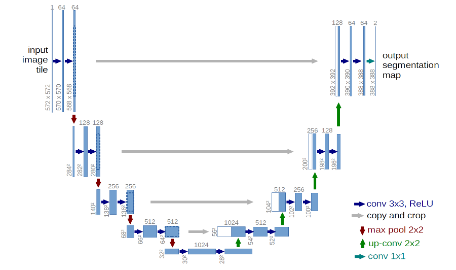Figure 4. U-net architecture

The paper was very clear and readable and I had a prototype running in mxnet without much effort. As someone that deploys deep learning systems to various targets (embedded, windows, linux, cloud etc) in various programming languages I really recommend this library.

After getting an example running I started to experiment with different parameters and settings. Below a few key observations and improvements are enumerated.

1. Segmentation nets are numerically unstable. I relied heavily on batch normalization.
2. Smaller batch sizes yielded better scores and stability. I settled for batchsize = 2.
3. Elastic deformations were by far the most effective augmentations
4. The shortcut connection gave a significant improvement in accuracy.
5. Logistic regression was better loss than RMSE but even better alternatives quite possibly exist.
6. Dropout helped but it was hard to determine where to apply it. I choose upstream after the shortcut merges.
7. Adding more layers quickly led to diminishing returns
8. Adding more filters per layer quicky showed no improvement
9. It was hard, if not impossible to overfit the network.
10. Training time was around 5 hours

After a lot of trial and error I ended up with the following network. Note that I used relu activations and batch normalization after every convolution. I used padding for the convolutional layers to not let them decrease output shape. Below the architecture is displayed. Note that my approach is very much trial and error and many decisions don’t have a grounded theory.

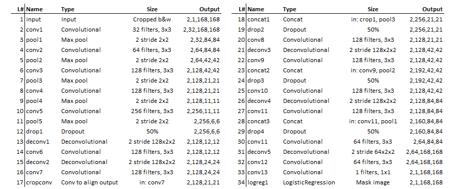Figure 5. Network definition used for this solution

The segmentation results were quite impressive. The “easy cases” where virtually perfect. Cases where the LV tissue was only half around were nicely filled up with a “half moon”-like overlay. There were some cases where the net was confused but this was almost always due to strange outliers of which it never had seen any examples before. Patients with many heavily contracted LV’s seemed to be a little underestimated by the system. This is probably because I should have labeled contracted LV’s more generous. Below, a few cases are shown.

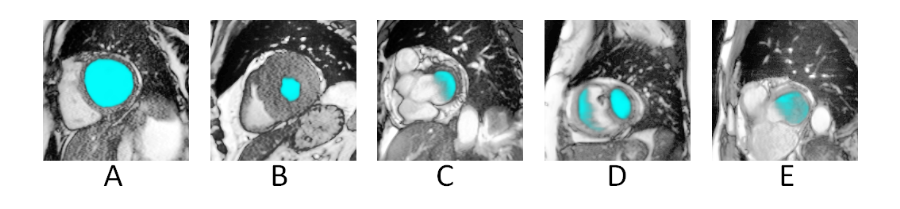Figure 6. Segmentation results. A. Normal. B. Heavy contraction. C. Chamber only partly surrounded by LV tissue D. and E. Uncommon cases where the u-net was confused.

Integrating the predictions into volumes and data cleaning.

Theoretically, once you have the LV areas per slice, the step to compute the volumes is straight forward. You take the slice areas and multiply by their thickness and then sum. You can even be more fancy and compute the volumes using frustum of a cone approximations like in the tutorials. I did that but it only gave a small improvement. It was much more beneficial to put extra effort in the data cleaning process. Taking MRI’s is obviously a very error prone process and many computations went wrong because of irregularities in the data. Below some common problems are discussed.

1. Patients with virtually no slices.
   Patient 595 and 599 only had 3 slices. I decided to drop them and predict their volumes later on based on averages for age and sex.
2. No real guide for slice thickness.
   I eventually used the difference between slice locations to determine the slice thickness. Although the slice location was not 100% perfect other calculations based on image orientation and location also had their problems so I settled for the simplest option.
3. Slice ordering.
   Usually the MRI makes slices from the base downto the apex. But sometimes the machines seemed to get stuck or went back up again. This would result in negative slice thicknesses. The fix was to order the slices based on location and not in time.
4. Out of range slices.
   After ordering the slices I sometimes noticed thicknesses of 100+ mm. Since the expected thickness was around 10mm I concluded that these slices were out of range (stomach, neck) so I dropped them.
5. Missing slices.
   After putting in a maximum slice thickness there turned out to be some sliced that were 20 or even more mm but they were valid. My conclusion was that in these cases other slices in the sequence were missing. My measure against this was to allow for these big slices as long as they fell between the base and the apex.
6. Wrongly oriented slices.
   In a very few occasions slices would suddenly be rotated. Luckily my segmenter did not suffer from this so there was no need to take measures against this.
7. Frames not present on all slices.
   Sometimes certain frames where not present in all slices. This could lead to errors in comparing the total volumes between frames. Therefore I introduced a requirement that a frame had to be present in every slice or else it would be dropped.

Another important point to note is that two volumes need to be determined at the same time. Namely systole (contracted) and diastole (expanded). I tried two approaches for determining which frames where systole and diastole. The first was to take the frame with total volume maximum volume as diastole and the one with the minimum volume as systole. The second method was to find the image with the larges area and use that frame as diastole. Then within that series look for the smallest area and use that frame as systole. The second approach is probably what doctors do but somehow the first approach was more stable and worked better with the calibration step that followed. My guess the reason is that the first approach is more consistent. It structurally a bit too low for systole and a bit too high for diastole. This signal can easily be picked up by the gradient boosting procedure that I used for calibrating the volumes.

Calibration

From the labels to the segmenter to the volume computation there were plenty of opportunities to introduce systematic errors. The traindata for the competition provided the “real” volumes as determined by the cardiac specialists. It would be wasteful to not use this data to improve the estimations. During a “calibration” step I tried to detect and mitigate systematic error by using a gradient boosting regressor with the raw estimations and some extra features. I tried a lot of features that had great potential for predicting the error. Examples are the amount of “unsureness” of my segmenter expressed in low probability pixels, the biggest slice, the number of dropped slices etc. However it turned out that the regular features provided in the dicom files were the most benefitial. Next to the raw predictions other helpful features were age, sex, angle, slice-thickness and slice-count.

There were a number of targets that could be regressed on. The volume, the real/estimated ratio and the error (residual). The last one gave the best improvements. The gradient boosting regressor tried to predict the error in the estimation given all the features. With the prediction of that error I could adjust my estimation and this led to a better overall estimation. To avoid the risk of overfitting it was necessary to train the segmenter in folds. For more information about two level models this is a nice guide. Training different folds slowed everything down quite a bit but in the end I think it was well worth the effort. Below is a table of the improvements in mean absolute errors.

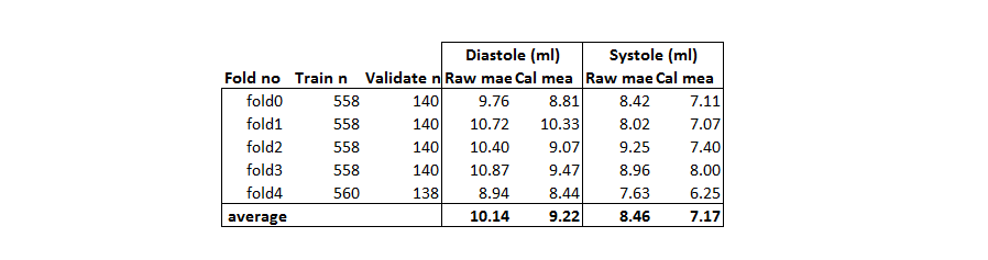Figure 7. Mean absolute error before and after calibration

As can be seen the MAE improved by 1 ml which was quite a bit. On the leaderboard the calibration step provided a boost in the score of around 0.0005 which is almost the difference between #3 and #4.

Submission

Kaggle came up with an evaluation function which I came to like very much. This was the Continuous Rank Probability Score. Next to an accurate prediction you also had to tell how sure you were of your prediction. I tried a few strategies but the one that worked best for me was the following. For a prection I determined the standard deviation in the errors for other prediction with similar volumes. Then I plugged the estimated volume and the standard deviation in a cumulative density function. The resulting values were used for my submission. This was a simple and stable procedure that was aware of errors/variance in the ground thruth and in the estimations. The ideal batch size for determining the standard deviation was between 30 and 60.

Some conclusions and remarks

First of all I’m very happy with the resulting model. It is simple and straightforward and there are a number of possible improvements if one were to use this model in a real-life scenario. Below are a number of possible improvements.

1. Hand-labeling by a real expert.
   I am sure that I labeled some of the cases completely wrong. Labels provided by experts would most likely drastically improve the performance.
2. Active learning (boost hard examples).
   I was afraid to boost the train images of cases where the segmenter had a hard time. People might accuse me of cheating. However active learning is a perfectly valid aproach for improving the performance of a system like this.
3. Cleaner data.
   The outliers in this dataset were very important in this competition. A small number of patients were responsible for the biggest loss in performance. Of course I investigated them thouroughly. However, in many cases I could not find a problem in my estimated volumes. My conclusion was that the provided volumes were plain wrong. The biggest outlier was patient 429. This patient alone was responsible for a 89ml error. Until now there is still no explanation for this strange value. Cases like this confused the calibration step and increased the standard deviation during the submission so they had a big impact on the final score.

Before the competition the doctors told during a Q&A session that errors 10ml would be acceptable. On average we are below this value. Of course there is the problem of the outliers but I am very confident that these issues can be resoved. Therefore I would like to call this problem:

Code

The code can be found here

Thanks

1. Kaggle and Booz Allen Hamilton.
   Thank you for organizing this complex and cool challenge. There were some complaints about the whole two phase setup and the quality of the data. But if we want to take on more ambitious problems than the usual CTR/forecasting stuff you sometimes need to try something new an take some risk.

2. Mxnet.
   What can I say… great library when you also want to deploy your systems in real-world situations. Especially good windows support is something that is severely lacking from most other libraries.

3. The authors of the U-net paper.
   The idea was great. The paper was easy to understand with clear language and concrete examples. That is something you do not find everyday in the deep learning community.