Summary

This document describes my part of the 2nd prize solution to the Data Science Bowl 2017 hosted by Kaggle.com. I teamed up with Daniel Hammack. His part of the solution is decribed here The goal of the challenge was to predict the development of lung cancer in a patient given a set of CT images. Detailed descriptions of the challenge can be found on the Kaggle competition page and this blog post by Elias Vansteenkiste. My solution (and that of Daniel) was mainly based on nodule detectors with a 3D convolutional neural network architecture. I worked on a windows 64 system using the Keras library in combination with the just released windows version of TensorFlow.

Initial familiarization and the resulting “plan of attack”

Before joining the competition I first watched the video by Bram van Ginneken on lung CT images to get a feel for the problem. I tried to manually asses a few scans and concluded that this was a hard problem where you almost literally had to find a needle in a haystack. Like described by Elias Vansteenkiste the amount of signal vs noise was almost 1:1000.000. As the first efforts on the forums showed, the neural nets were not able to learn someting from the raw image data. There were only 1300 cases to train on and the label “Cancer Y/N” was to distant from the actual features in the images for the network to latch upon.

The solution would be to spoonfeed a neural network with examples with a better signal/noise ratio and a more direct relation between the labels and the features. Luckily the competition organizers already pointed us to a previous competition called LUNA16. For this dataset doctors had meticulously labeled more than 1000 lung nodules in more than 800 patient scans. The LUNA16 competition also provided non-nodule annotations. So when you crop small 3D chunks around the annotations from the big CT scans you end up with much smaller 3D images with a more direct connection to the labels (nodule Y/N). The dataset also contained size information. As the size usually is a good predictor of being a cancer so I thought this would be a useful starting point.

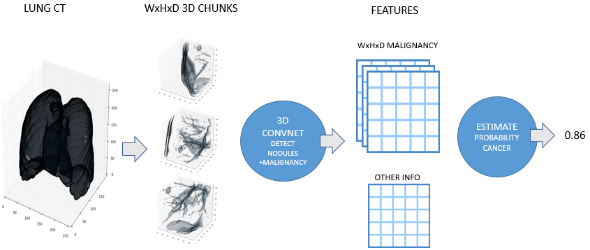
Figure 1. High level description of the approach

Later I noticed that the LUNA16 dataset was drawn from another public dataset LIDC-IDRI. It turned out that in this original set the nodules had not only been detected by the doctors but they also gave an assessment on the malignancy and other properties of the nodules. This malignancy assessment turned out to be learnable by the neural network and a “golden” feature for estimating the cancer risk.

The final plan of attack was to train a neural network to detect nodules and predict the malignancy of the detected nodules. During prediction every patient scan would be processed by the network going over it in a sliding window fashion. This resulted in a lattice containing malignancy information for every location that the sliding window had visited. The final step was to estimate the chance that that the patient would develop a cancer given this information and some other features.

Preprocessing and creating a trainset

It was important to make the scans as homogenous as possible. To do this, first every scan was rescaled so that every voxel represented an volume of 1x1x1 mm. Both Daniel and me did some experiments with other scales but 1mm was a good balance between accuracy and computational load. With CT scans the pixel intensities can be expressed in Hounsfield Units and have semantic meaning. As suggested on the forums all intensities were clipped on the min, max interesting hounsfield value and then scaled between 0 and 1. The last importand CT preprocessing step was to make sure that all scans had the same orientation.

Almost all the literature on nodule detection and almost all tutorials on the forums advised to first segment out the lung tissue from the CT-scans. However, none of the segmentation approaches were good enough to adequately handle nodules and masses that were hidden near the edges of the lung tissue. Sometimes these were removed from the images leaving no chance for the nodule detector to find. I first considered training a U-net to properly segment the lungs. This would almost surely give better results than traditional segmentation techniques. However, as a human inspecting the CT scans, borders of the lung tissue gave me a good frame of reference to find nodules. It was my hunch that the convnet might also “like” this information. So in the end I decided to train and predict on raw images. After some tweaking with the traindata this worked fine and did not seem to have any negative effects.

In more straight forward competition the traindata is a given and is not interesting to discuss. However, for this solution engineering trainset was an essential, if not the most essential part. I used provided labels, generated automatic labels, employed automatic active learning and also added some manual annotations. Below is a table with the different sources that were used as labels.

Table 1. Labelsets used for training.

The quantity of positive doctor labels from LIDC is five times the number of the LUNA16 set. The reason is that these are the combined annotations of 4 doctors. So one nodule can be annotated 4 times. LUNA16 also ignored nodules that were only annotated by less than 3 doctors. I decided to keep these ignored nodules in the training set because of the valuable malignancy information that they provided.

The candidates(v2) labelset was taken straight from LUNA16. These were false positive candidate nodules taken from a wide range nodule detection systems. Note that some of these candidates overlapped nodules that were tagged by less than 3 doctors. I kept them in to provide some counter balance against those posibly false positive nodules.

To train on the full images I needed negative candidates from non-lung tissue. I used a simple lung segmentation algorithm from the forums and sampled annotations around the edges of the segmentation masks. This was enough to teach the network to ignore everything outside the lungs.

After doing a first training round I predicted nodules on the LUNA16 datasets. All false positives were harvested and added to the trainset.

Later in the competition I wanted to build a second model. For this extra model I played radiologist and let the network predict on the NDSB trainset. Then I manually tried to select interesting positive nodules from cancer cases and false positives from non-cancer cases. Then I trained a second model with these extra labels. I expected better results but it turned out that I am a bad radiologist since the second model with my manual labels was worse than the model without. However, the blend of the two models was better than the seperate models so I kept the second model in.

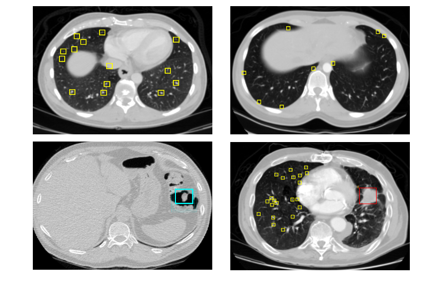
I used a special, hastily built, viewer to debug all the labels. While viewing I noticed that some >3cm big nodules were ignored by the doctors. Reading the LIDC documentation I found that the doctors were ordered to ignore >3m labels. Fearing that my classifier would be confused by these ignored masses I removed negatives that overlapped with them. Below are some screenshot I took.

Figure 2. Label visualizations. Top left: Luna16 candidates, Top right: Non lung tissue edge, Bottom left: A false positive, Bottom right: Non annotated mass I removed candidates around.

3D convnet training strategy and architecture

Even with a better trainset it still took considable tweaking to effectively train a neural network. The dataset was still heavily imbalanced (5000:500000) and there was much variation in size and shape of the positive examples. I had considered U-net architectures but 2D U-nets could not exploit the inherently 3D structure of the nodules and 3D U-nets were quite slow and inflexible. The main reason to skip U-nets was that it was not necessary to have a fine-grained probability map but just a coarse detector. Having a small 3D convnet that you slide over the CT scans was much more lightweight and flexible.

My first goal was to train a working nodule predictor. The first thing I did was to upsample the positive examples to a ratio of 1:20. For generalization a number of augmentation strategies were tried but somehow only loss-less augmentations helped. In the end I used heavy translations and all 3D flips.

Once the classifier was in place I wanted to train a malignancy estimator. The provided malignancy labels ranged from 1 (very likely not malignant) to 5 (very likely malignant). To put more weight on the malignant examples I squared the labels to a range from 1 to 25. At first I was thinking about a 2 stage approach where first nodules were classified and then another network would be trained on the nodule for malignancy. To win time I tried one network to train both at once in a multi-task learning approach. This worked quite well and since the approach was quick and simple I decided to go fo this.

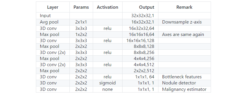
Usually the architecture of the neural network is one of the most important outcomes of a competition or case study. For this competition I spent relatively little time on the neural network architecture. I think this is mainly that there are already so many good baseline architectures. I started out with some simple VGG and resnet-like architectures. All performed roughly the same. Then I wanted to try a pretrained C3D network. The pretrained weights did not help at all but the architecture without pretrained weights gave a very good performance. The final architecture was basically C3D with a few adjustments.

The first adjustment was the receptive field which I set to 32x32x32 mm. This might sound like a bit too small but it worked very good with some tricks later in the pipeline. The idea was to keep everything lightweight and make a bigger net on the end of the competition. But since Daniel’s network was 64x64x64 mm I decided to stay at the small receptive field so that we were as complementary as possible. The second adjustment I made was to immediately average pool the z-axis to 2mm per voxel. This made the net much lighter and did not effect accurracy since for most scan the z-axis was at a more coarse scale than the x and y axes. Finally I introduced a 64 unit bottleneck layer on the end of the network. The was to do some experiments with training on the raw intermediate features instead of the predicted malignancy later in the process.

Table 2. Network architecture.

Spicing things up: strange tissue detector

Looking at the forums I had the feeling that all the teams were doing similar things. I was looking to get an edge by doing something “out of the box”. While looking at the scans some other thing occurred to me. Like with the LUNA16 dataset much of the effort was focused on lung nodules. However, when a cancer develops they become lung masses or even more complicated tissues. I noticed that when a scan had a lot of “strange tissue” the chance that it was a cancer was higher. Also, on a lot of these scans, my nodule detector did not find any nodules. This gave some pretty bad false negatives.

Note that this were only ~10 cases in the trainset of which ca. 5 were cancer cases. Still I thought it was worth the effort to detect the amount of strange tissue on a scan to hedge against these hard false negatives. Luckily LUNA16 contained a lot of such cases so I quickly labeled examples and trained a U-net. The tissue detector worked surprisingly well and both local CV and LB improved a little for me. It is hard to say exactly how much because it varied between models but I would like to think it gave me around 0.002-0.005. For this improvement and, to be honest, because I thought it was a cool addition I kept it in. Below are some example cases.

Figure 3. Strange tissue examples highlighted.

I also tried to build an emphysema detector. Basically emphysema are smokers lungs. Doctors on the forum all claimed that when emphysema are present the chance on cancer rises. There were some easy algorithms published on how to assess the amount of emphysema in a CT scan. It came down to scanning on the image for areas containing around −950 hounsfield units. However, this approach did not work for me on the provided CT scans. Then I labeled some examples to train a U-net. This worked better but I got no real improvement on my local CV. My guess is that many cases in the dataset were scanned because there was something wrong with the lungs and therefore there were a lot of emphysema cases regardsless of lung nodules and cancer. I am not sure about this claim though. Perhaps I just did something wrong.

Final step cancer prediction

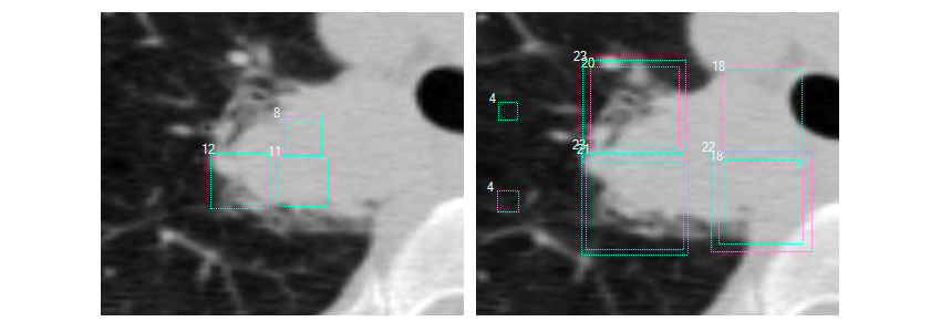
Once the network was trained the next step was to let the neural network detect nodules and estimate their malignancy. The CT-viewer that I built proved very useful for viewing the results. My conclusion was that the neural network was doing an impressive job. It picked up many nodules that I completely overlooked while I saw only very few false positives. There was only one serious problem. It missed some obvious very big nodules. For scoring false negatives had the most negative effect sometimes giving a 3.00 logloss. As a small expreriment I tried to downsample the scans 2 times to see if the detector then would pick up the big nodules. Remarkably it did and it worked quite well. Therefore I adjusted the pipeline to let the network predict at 3 scales namely 1, 1.5 and 2.0. This took considerably more time but it was worth the effort.

Figure 4. Large nodule not well estimated at 1x zoom (left) while having been processed at 2x zoom (right) it is much better. Size of the rectangles indicates estimated malignancy.

Given this data and some extra features I wanted to train a gradient boosting classifier to predict the development of cancer within one year. All this was relatively straight forward. The main problem was that the leaderboard was based on 200 patients and contained, by accident, a big number of outlier patients. After some tweaking my (1000 fold!) local cross validation was roughly 0.39-0.40 on average while the leaderboard score varied between 0.44 and 0.47. The problem was that is was very hard to relate the leaderboard score to the local CV. Improvements on local CV could result in much lower LB scores and visa versa.

I spent a lot of time trying to “fix” the local CV/leaderboard compass. I did not succeed in this and as a result I only used techniques and features that improved both CV and LB. The reason was because this was a two stage competition and there was a slim chance that the stage 2 data would look more like the LB dataset than the actual trainset. Many teams seemed to have bet on this since, as it turned out, there was a lot of LB overfitting going on. In the end I only used 7 features for the gradient booster to train upon. These were the maximum malignancy nodule and its Z location for all 3 scales and the amount of strange tissue.

For ensembling I had two main models. The first model was trained on the full LUNA16 dataset. For the second I tried to apply active learning by selection hard cases and false positives from the NDSB trainset. As I am no radiologist I tried to play it on safe only selecting positive examples from cancer cases and negative examples from non cancer cases. I did something wrong anyway since the second model scored worse than the LUNA16 only variation. Combined together by averaging they gave a good boost on the LB and also improved local CV significantly.

Teaming up with Daniel Hammack

When doing machine learning competitions it’s usually a good idea to combine solutions from different angles. I already worked together with Daniel in a previous medical competition and knew he was an incredibly bright guy. Also his “style” of doing machine learning differs from mine. His angle is more from a research point of view while I am more an engineering guy. When we contacted we were both pretty sure that we had an 100% original solution and that our approaches would be highly complementary.

Once we joined at first we were slightly disappointed that we both had exactly the same insight to use the malignancy information from the LIDC dataset. From that aspect our solutions turned out to be very similar. However, luckily the rest of the design choices and approaches where completely different leading to a significant improvement on the LB and local CV. Below some of the major differences are enumerated.

Table 3. Differences between Julian and Daniel.

Joining forces was a very good decision. While I was heavily frustrated with the leaderboard Daniel was quite confident that we should mainly focus on local CV. So in the end I reduced the effort in matching local CV with LB and focused on improving the local CV a bit more. On the final leaderboard this turned out to be a good decision since the final stage2 leaderboard matched quite well with local CV and we ended up second. This while many teams with a better stage 1 leaderboard score turned out to have been overfitting.

Conclusions and remarkss

When looking at the predictions on the CT scanes we think that the resulting model performs very well. The ROC AUC was 0.85 for the stage 1 public leaderboard (~0.43 logloss) and is be even better for the stage 2 private dataset (0.40 logloss). An exciting question would be how good a trained radiologist would do on this dataset.

Regardsless of the outcome, automatic nodule detection can be a big help for radiologists since they nodules can easily be overlooked. The malignancy assesments are good but they were based on only 1000 examples so there should a lot of room for improvement.

The solutions of both Daniel and mine took considerable engineering and many steps and decisions were made ad-hoc based on experience and gut feeling. There was simply not enough time to properly test the effects of all options. Below some suggestions for further research are made.

• Establish a radiologist baseline.
  It would be very interesing to see establish a baseline on how well a radiologist performs on this dataset.
• Malignancy labeling of the NDSB dataset.
  For this competition we only had ~1000 nodules to train on. Having more, precisely labeled examples would certainly improve the algorithm even more.
• Try out more neural network architectures.
  I spent very little time on figuring out which network architecture worked best. It might well be that some much better performing configurations were missed.

Code

The code can be found here

Thanks

1. Kaggle and Booz Allen Hamilton.
   Thank you again for organizing this complex and relevant challenge. Next to the fun of the competition I really had the feeling I was doing something “good” for society.

2. Authors of Keras and TensorFlow.
   The windows release of TensorFlow came just at the right time for me. The Keras API was very easy to use.

3. Daniel Hammack.
   In CV we trust!